A delivered scene is raw material, not an answer. SatView runs it through a real processing
chain today; with v3 it reads it too — with models you control, on hardware you own.
04 · Process
Build the chain visually, run it asynchronously
A pipeline is a DAG you assemble in the browser. Jobs are submitted to the Python backend,
tracked in the interface, and their outputs land back on the map as layers.
30+ native operations
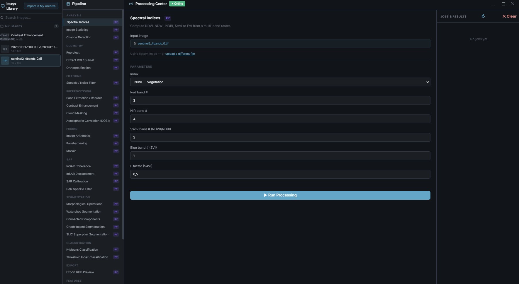
Grouped by intent in the Processing Center: analysis (spectral indices, image statistics, change detection), geometry (reproject, extract ROI, orthorectification), filtering, pre-processing (band extraction, contrast enhancement, cloud masking, atmospheric correction DOS1) and fusion (image arithmetic, pansharpening, mosaic).
SAR & interferometry
SAR calibration, speckle filtering, and interferometric processing as first-class pipeline steps: InSAR coherence and InSAR displacement. Range-Doppler terrain correction is on the roadmap.
Classification & segmentation
K-means and threshold-index classification, morphological operations, watershed, graph-based and SLIC superpixel segmentation, connected components — each producing a labelled raster you can carry downstream.
Orfeo Toolbox & ESA SNAP
Industry-standard remote sensing toolchains driven through their CLI and GPT interfaces — not reimplemented, actually invoked.
Cloud-native
Process straight from a COG URL without downloading the full scene first, and push results back as cloud-optimized GeoTIFF.
Super-resolution
Upscaling for detail recovery on lower-GSD sources, available as a pipeline step like any other operation.
Processing Center · operation catalogue and job parameters
05 · Analyze
Inference that produces geometry, not just pictures
Every AI job returns a raster and a companion GeoJSON reprojected to WGS84 — so results
are map layers, queryable objects and exportable evidence, not screenshots.
Coming in SatView v3. The inference chain described below is in development.
The operations already appear in the Processing Center; the models, the map layer and the
detection index ship with v3. Everything else on this page runs today.
Object detection — ONNX models run with a sliding window, or classic blob detection. Classes: vehicle, ship, aircraft, building, storage tank. Output: heatmap raster plus GeoJSON.
Change detection — Change Vector Analysis with Otsu thresholding, polygonized into vector change masks.
Semantic segmentation — ONNX models or spectral K-means, producing a labelled raster with its legend.
Detection layer — results rendered on the map as a GeoJSON layer, alongside the imagery they came from.
Auto-indexing — every detection feeds a searchable index, so “show me every ship detected in this area last month” becomes a query rather than a manual review.
Bring your own models — upload, version and manage your own ONNX weights. Nothing is locked to a vendor's model zoo, and no model choice is imposed on you.
AI Vision — a multimodal model describes the scene and answers questions about it.
Natural-language query — plain English translated into catalog search parameters.
Where the models run matters. Inference happens on your Python backend, on your
hardware. Imagery is not uploaded to a third-party inference API unless you explicitly configure
one for AI Vision or natural-language query.
Exploitation
Reading the results
Time Series Viewer
Swipe comparison between acquisitions across a date range.
InSAR viewer
Reads back the coherence and displacement products as map layers.
Content search v3
Query the index of detected objects, with results on the map and in a list. Arrives with the detection chain it depends on.
Intel reports
Generate a report and export it to PDF with cover page, tables and classification banner.
Now make it run without you
Monitoring rules turn this chain into a standing watch — re-acquiring on cadence, or retrying when cloud or quality fall short.